Statistical analysis / Investment prioritisation / Innovation ecosystems
Prioritise business capability in the innovation investment agenda
A cross-country statistical case that turns innovation indicators into a cautious investment agenda, with explicit separation of association and policy impact.

The recommendation
Use cross-country evidence to choose what to investigate and test locally.
The 2025 GII analysis supports examining firm capability, infrastructure and market conditions together when designing innovation programmes. Business Sophistication has the strongest positive standardised association with Knowledge and Technology Outputs after controlling for the other modelled input pillars. This supports a commercialisation-focused diagnostic agenda, but does not establish that reallocating a given budget will cause a specified output gain. Translate the associations into targeted programme hypotheses, then fund local pilots with outcome evaluation.
Decision at stake
How an innovation agency should prioritise diagnostic work and pilot funding without treating a cross-sectional regression as a causal allocation formula.
An individual Statistical Decision Making assignment using the 2025 GII. Core descriptive, comparison and regression findings were recomputed from the supplied SPSS-ready workbook and checked against the archived official-source workbook.
Evidence and decision parameters
- Economies analysed
- 139
- 2025 GII cross-section; complete observations for the outcome and five regression predictors.
- In-sample variance explained
- 83.9%
- Reported regression R², reproduced from the supplied workbook; this is not a policy impact estimate.
- Business Sophistication β
- 0.605
- Strongest positive standardised partial coefficient in the specified five-predictor model.
Move from rankings to an investable question
Innovation rankings show relative position, while investment decisions require a diagnosis of the constraints preventing knowledge from becoming economic output. The assignment examined whether income groups differ in Knowledge and Technology Outputs and which innovation-system conditions are associated with those differences. The consulting question is how to turn that evidence into a disciplined programme agenda.
The unit of analysis is an economy. The outcome is the GII Knowledge and Technology Outputs pillar, with Institutions, Human Capital and Research, Infrastructure, Market Sophistication and Business Sophistication as predictors. Selecting an output pillar avoids regressing the overall GII score on its own input components, although composite measures and shared structural factors still constrain interpretation.
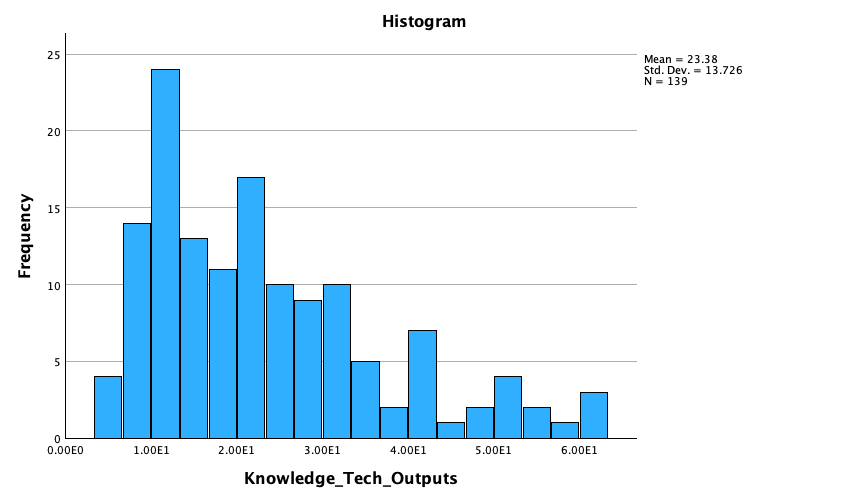
Figure 1. Innovation output is unevenly distributed across economies
The original distribution establishes the analytical baseline: a mean output score of 23.38 masks a substantial spread and a positively skewed cross-country profile.
Interpretation: This is a 2025 GII cross-section, not a trend or a measure of programme impact.
Source: SDM_WIPO_GII_2025_Final_Report_REVISED.docx · Figure 3 · Original SPSS output
Income is strongly associated with output, but is not a programme design
The report finds an average output score of 33.94 for high-income economies and 16.67 for the workbook’s non-high-income group. Unequal variances led to a Welch comparison, which was statistically significant. The four-group analysis also used a robust Welch procedure; high-income economies exceeded each of the other income groups, while upper-middle and lower-middle differences were not statistically significant.
These differences establish an important baseline, without telling a policymaker which intervention to buy. Richer economies differ in industrial composition, accumulated research, market access and many unmeasured conditions. Peer comparisons should therefore consider economic structure and capabilities. Selecting only top-ranked economies as templates could prescribe institutions or infrastructure that a local programme cannot reproduce.
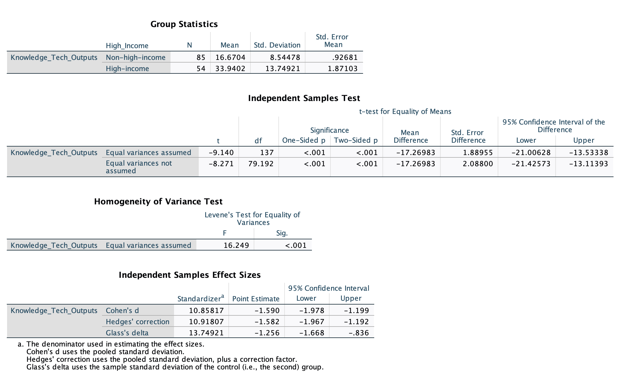
Figure 2. The high-income comparison shows a substantial output gap
Use the unequal-variances row because Levene’s test rejects equal variances. Reversing the original SPSS subtraction order, high-income economies score 17.27 points higher on average, with a 95% confidence interval of 13.11–21.43 points.
Interpretation: The binary non-high-income category includes one economy with unknown income classification, coded 0 in the source workbook. This comparison needs sensitivity testing with that case excluded. The difference is observational, not a causal effect of income or an intervention.
Source: SDM_WIPO_GII_2025_Final_Report_REVISED.docx · Table 4 · Original SPSS output
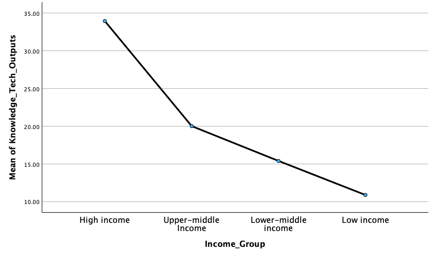
Figure 3. Income-group means provide a baseline for peer comparison
The four-group profile makes the scale of the observed income gradient visible. It supports more careful peer selection before diagnosing a local innovation constraint.
Interpretation: The four-group analysis excludes the economy with unknown income classification (N = 138). The connecting line joins categories; it does not show change over time or demonstrate that moving income groups causes an output gain.
Source: SDM_WIPO_GII_2025_Final_Report_REVISED.docx · Figure 5 · Original SPSS output
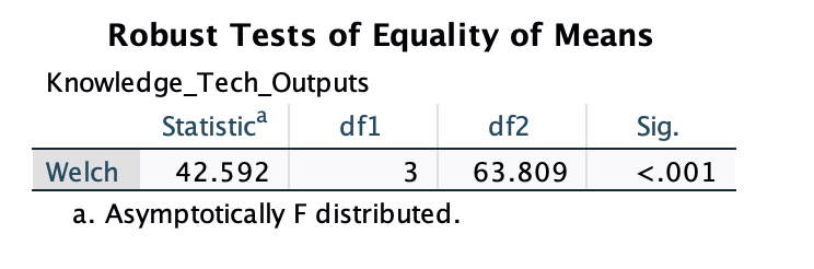
Figure 4. The income-group difference survives an unequal-variance test
The original Welch result rejects equality of the four income-group means, F(3, 63.81) = 42.592, p < .001. It establishes a group-level association without identifying a policy instrument.
Interpretation: The unclassified economy is excluded (N = 138). This omnibus result does not imply that every pair of income groups differs; the report’s Games–Howell comparison finds no significant upper-middle versus lower-middle difference.
Source: SDM_WIPO_GII_2025_Final_Report_REVISED.docx · Table 6, robust test · Original SPSS output
Business capability is the leading signal in the specified model
The five-predictor model explains 83.9% of the observed sample variation, with adjusted R² of 83.2%. Business Sophistication has the largest positive standardised coefficient at 0.605, followed by Infrastructure at 0.270 and Market Sophistication at 0.177. Human Capital and Research is not a statistically significant unique predictor in this specification, despite its plausible importance within the broader system.
The decision implication is to investigate the connections between firms, research, infrastructure and finance. A programme could test whether firms face commercialisation, collaboration or adoption barriers before adding another stand-alone input subsidy. The coefficients cannot prescribe budget percentages, compare intervention returns or imply that human-capital investment is unnecessary.
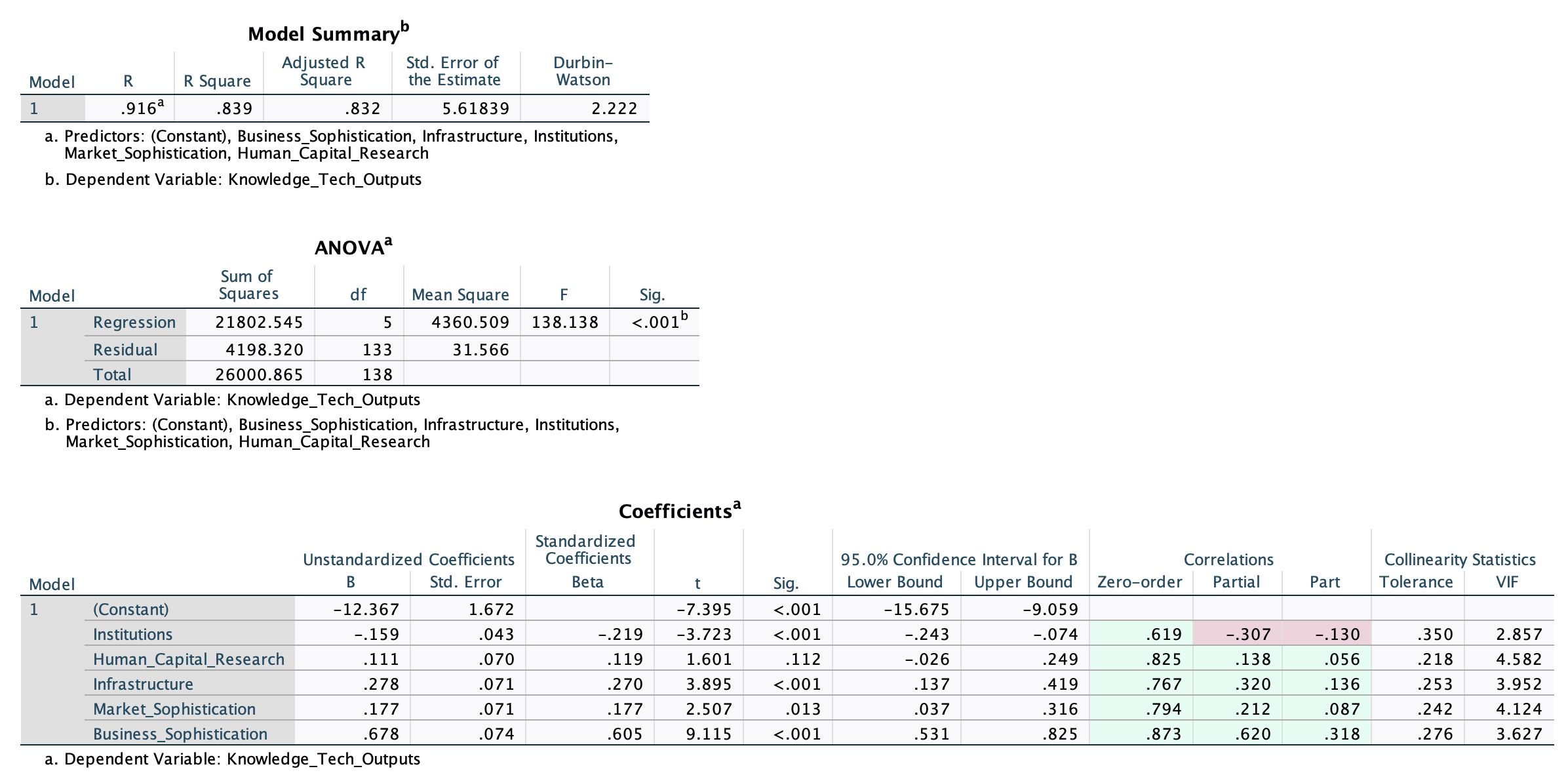
Figure 5. Business Sophistication is the leading positive partial association
The five-predictor model explains 83.9% of the observed in-sample variation. Business Sophistication has the largest positive standardised coefficient (β = 0.605), making firm capability and commercialisation useful areas for local diagnosis.
Interpretation: These are conditional associations between composite indicators, not causal effects or budget weights. Correlated predictors and the negative partial Institutions coefficient require caution; the output also shows its positive zero-order correlation. Human Capital and Research is not significant in this specification. Open the original image to inspect the full coefficient table.
Source: SDM_WIPO_GII_2025_Final_Report_REVISED.docx · Table 7 · Original SPSS output
Resolve the interpretation traps before recommending policy
Institutions has a positive simple correlation with output, yet a negative partial regression coefficient. The report records overlapping predictors, with variance inflation factors from 2.857 to 4.582. This reversal may reflect shared variance or suppression; it provides no defensible basis for weakening institutions. Likewise, a high in-sample R² does not demonstrate reliable prediction in a new economy or year.
Income coding also requires care. One economy has no income-group classification but is coded into the binary non-high-income category. The report excludes it from the four-group comparison but includes it in the binary tests. A decision-ready extension should rerun those comparisons with the unclassified case excluded and document sensitivity before relying on the precise income-gap estimates.
Build a programme portfolio around a verified local bottleneck
A broad infrastructure programme may address enabling constraints, but can absorb resources without changing firm behaviour. General research subsidies can expand knowledge creation while leaving commercial pathways unresolved. A firm–research collaboration programme more directly tests the leading model signal, but requires capable participants, useful projects and evidence that public support changes activity rather than subsidising existing plans.
The proposed approach combines a local constraint diagnostic with a bounded collaboration or technology-adoption pilot. Interview firms and research partners, map referral and procurement barriers, and establish demand for the proposed support. Choose the intervention from that evidence; the cross-country analysis identifies areas worth testing rather than proving a universal solution.
Measure additional economic activity rather than programme volume
Track progression from participation to collaboration agreements, prototypes, adoption and commercial revenue, using measures suitable to the intervention. Count applications or workshops as delivery indicators, with value assessed through additional capability and outcomes. Record firm investment and support cost so an evaluator can compare programme efficiency across cohorts.
Establish the counterfactual before launch. Where feasible, randomise a phased rollout; otherwise use comparable non-participants and a documented baseline, acknowledging selection bias. Follow outcomes long enough for commercialisation to occur. Annual GII ranking movement is too broad and method-dependent to attribute to a single pilot, so retain it as context rather than a contractual success measure.
Supporting evidence
Additional charts and frameworks from the source study.
Figure 6. A categorical test reinforces the income–output association
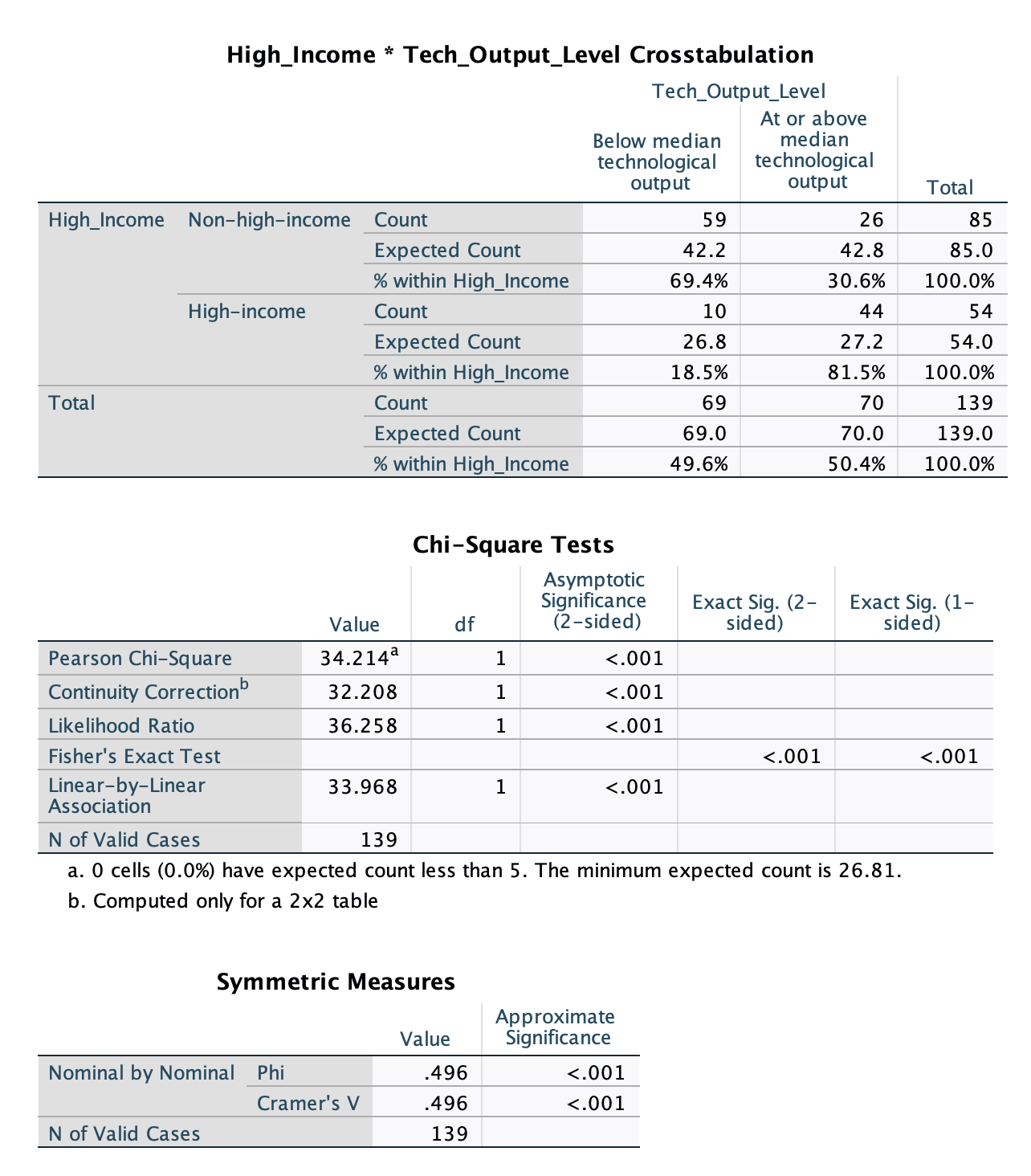
Figure 6. A categorical test reinforces the income–output association
The source cross-tabulation compares income status with a median-based output category. No expected cell count falls below five, and the reported association is substantial (Cramér’s V = 0.496).
Interpretation: The non-high-income category includes the unknown-income economy coded 0 (N = 139), so sensitivity analysis remains necessary. The median split simplifies a continuous score and does not establish causality.
Source: SDM_WIPO_GII_2025_Final_Report_REVISED.docx · Table 5 · Original SPSS output
Figure 7. Group sizes and unequal variances explain the test choice
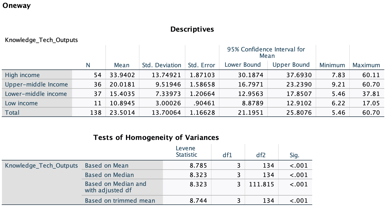
Figure 7. Group sizes and unequal variances explain the test choice
The source output provides group counts, means, dispersion and confidence intervals. Unequal group sizes and a significant Levene result support using the Welch test rather than an equal-variance comparison.
Interpretation: One economy with unknown income classification is excluded (N = 138). The low-income group contains 11 economies; the groups are not interchangeable samples of programme participants.
Source: SDM_WIPO_GII_2025_Final_Report_REVISED.docx · Table 6, descriptives and homogeneity tests · Original SPSS output
Figure 8. The raw output distribution departs from normality
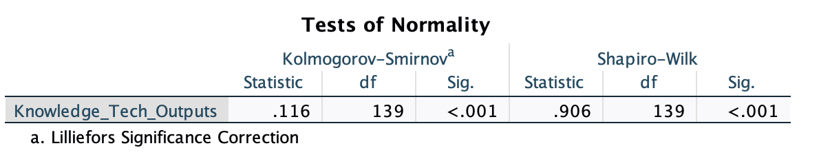
Figure 8. The raw output distribution departs from normality
The reported Shapiro–Wilk result (W = 0.906, p < .001) corroborates the skew visible in the histogram and supports caution when interpreting distributional assumptions.
Interpretation: This tests the raw outcome, not the regression residuals. A non-normal outcome alone does not establish that a regression model is invalid.
Source: SDM_WIPO_GII_2025_Final_Report_REVISED.docx · Table 3 · Original SPSS output
Figure 9. The outcome’s Q–Q plot shows departures in the tails
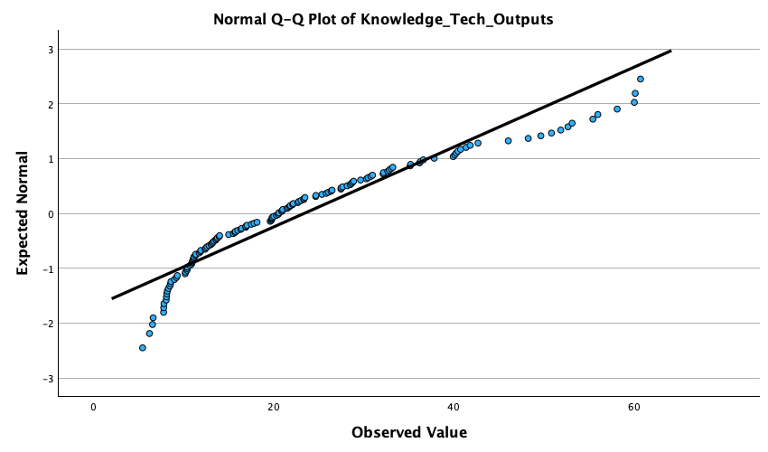
Figure 9. The outcome’s Q–Q plot shows departures in the tails
The original Q–Q plot provides a visual counterpart to the normality test, showing that the cross-country outcome does not closely follow a normal distribution throughout its range.
Interpretation: Outcome-distribution checks and regression-residual checks answer different questions.
Source: SDM_WIPO_GII_2025_Final_Report_REVISED.docx · Figure 4 · Original SPSS output
Figure 10. Residuals broadly follow the normal reference line
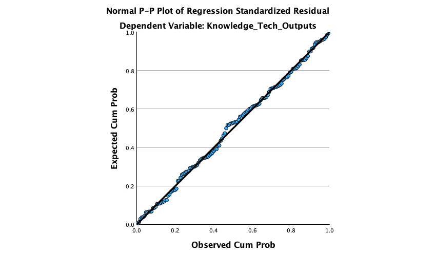
Figure 10. Residuals broadly follow the normal reference line
The report’s regression P–P plot is broadly consistent with approximate residual normality, even though the raw outcome distribution is skewed.
Interpretation: This visual check does not establish model stability, validate an intervention effect or replace sensitivity analysis.
Source: SDM_WIPO_GII_2025_Final_Report_REVISED.docx · Figure 6 · Original SPSS output
Figure 11. Residual scatter supports a cautious specification check
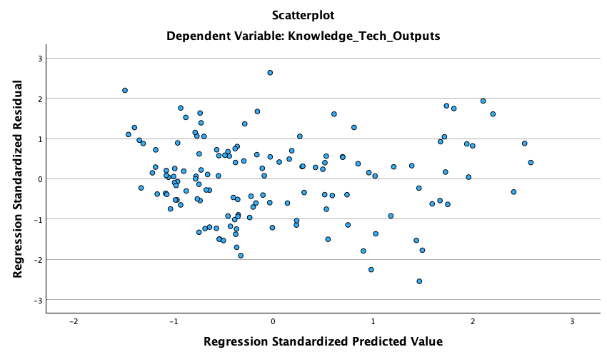
Figure 11. Residual scatter supports a cautious specification check
The original scatterplot shows no severe curved or funnel pattern identified in the report. It provides supporting evidence for the chosen linear specification and approximate constant residual variance.
Interpretation: Visual diagnostics cannot rule out omitted variables, influential observations, reverse causality or poor performance in another economy or year.
Source: SDM_WIPO_GII_2025_Final_Report_REVISED.docx · Figure 7 · Original SPSS output
Strategic priorities
Use the model to focus diagnosis
Ask how firms connect to research, infrastructure and markets. Validate the local bottleneck before selecting an instrument or committing a larger budget.
Complete robustness work before operational use
Resolve unknown income coding, examine influential cases and alternative specifications, and assess out-of-sample performance. Treat composite-pillar coefficients as associations.
Attach an evaluation design to pilot funding
Specify the expected behavioural change, comparison group, measurement window and cost per additional outcome before programme recruitment begins.
Path to implementation
Proposed sequencing and decision gates.
Months 1–2 · Proposed
Audit and contextualise the evidence
Agency analytics lead resolves coding, tests model sensitivity and compares relevant peer economies and local industry structure.
Decision gate: Documented robustness and a clearly bounded interpretation support proceeding to local diagnosis.
Months 2–4 · Proposed
Identify the binding programme constraint
Programme director and industry partners interview firms and researchers, assess existing support and define an intervention hypothesis.
Decision gate: A specific unmet need, participant demand and plausible route to additional activity justify pilot design.
Months 4–6 · Proposed
Fund a measurable pilot
Programme and evaluation teams agree eligibility, baseline data, comparison design, milestones and support costs before recruitment.
Decision gate: Evaluation feasibility, delivery capacity and participant commitments precede disbursement.
Months 6–18 · Proposed
Evaluate, adapt and decide on scale
Independent evaluators assess additional collaboration, adoption and commercial outcomes over a suitable follow-up period.
Decision gate: Evidence of additional value and delivery economics supports continuation, redesign or closure.
Value and measurement
The completed academic analysis provides reproducible evidence of cross-country differences and conditional associations. The portfolio case adds a source-data integrity check and a practical route from statistical insight to evaluated programme design. No policy implementation, causal effect or national innovation improvement is claimed.
Sources and scope
This is an observational cross-section of composite indicators, with different underlying data years and potential omitted variables, reverse causality and correlated predictors. Income coding needs sensitivity analysis. Economies are not a random sample of interchangeable programme participants. Regression diagnostics and significance do not establish causal impact, and proposed pilots remain untested.
Completed statistical report
APU Assignments.zip → Statistical Decision Making_Assignment → SDM_WIPO_GII_2025_Final_Report_REVISED.docx. Reported findings and analytical limitations.
Archived data and integrity check
WIPO_GII_2025_SPSS_Ready_139_Cases.xlsx and GII_2025_Exhaustive_Official_Dataset.xlsx. All six model variables matched across 139 economies; principal descriptive, Welch, chi-square and regression results were recomputed during portfolio preparation.
- WIPO · Global Innovation Index 2025 (opens in a new tab)
Primary publication for the historical 2025 analysis; this case does not claim to use the latest release.
- WIPO · Conceptual and measurement framework (opens in a new tab)
Primary methodology explaining economy coverage, composite pillars and underlying data-year limitations.
- WIPO · Sources and definitions (opens in a new tab)
Primary definitions supporting interpretation of the innovation-system and technological-output measures.
Continue reading
Related case studies
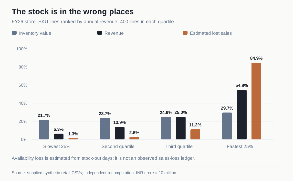
Retail operations / Profitability analytics / Inventory optimisation
Retail Operations Transformation & Profitability Optimisation
An end-to-end retail profitability diagnosis connecting store economics, assortment, inventory and a staged investment case across a simulated 20-store chain.
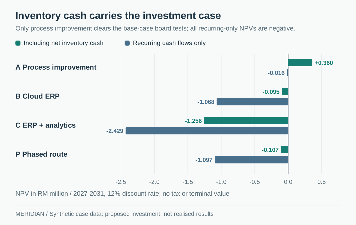
ERP investment / Operations transformation / Financial modelling
Meridian Precision Components: Make the ERP earn its place
A process-first manufacturing transformation strategy that tests an ERP investment against operational evidence, working-capital economics and production risk.
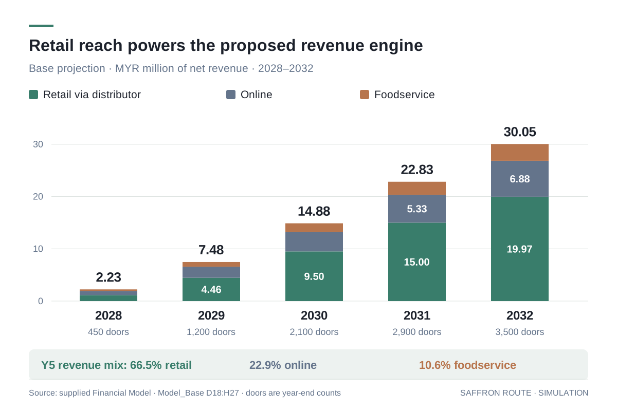
Market entry / Financial modelling / Commercial strategy
Saffron Route Foods: a staged route into Malaysia
An evidence-led market-entry case connecting consumer segmentation, distributor economics and a five-year financial model to explicit investment gates.